[This is a document created 8.7.2026 by Claude Fable AI in response to my request to derive formulas for calculating the dual determinant formulas for a Penrose cube with a rank-3 starting conic $S_0$. Typewriter font refers to elements of the software infrastructure I have been constructing with Claude’s help. Text in typewriter font refer to elements of the infrastructure for the Penrose cube software. -cg]
Dualizing the Penrose Determinantal Parametrization #
How the 4×4 parameter matrix of PenroseDeterminants.js transforms under
projective duality (point-wise ↔ line-wise conics), in the all-rank-3 case.
Companion to PENROSE_8_CONIC_THEOREM.md; read that first for the cube
combinatorics and the primal parametrization.
1. Setting #
The existing pipeline is entirely point-wise: a conic is a symmetric 3×3 form Q with incidence PᵀQP = 0 on points. Its dual — the envelope of tangent lines — is the line-wise conic Q* with mᵀQ*m = 0 on line coordinates, where Q* is the adjugate (cofactor) matrix of Q. Since Q is symmetric, Q* is symmetric too (no transpose subtlety), and
Q · Q* = det(Q) · Id
so Q* is projectively equivalent to Q⁻¹ while remaining polynomial in Q’s
entries — no division, consistent with the homogenization/LCD discipline of
PenroseDeterminants, and well-defined even where Q⁻¹ is not.
The mixed-determinant machinery in PenroseDeterminants.js is
type-agnostic: it never asks whether matrix[0][0] is a point-wise or a
line-wise conic, or whether the matrix[0][j] 3-vectors are lines or points.
Feeding it the dual data (S0*, pⱼ*, dⱼ*, aⱼₖ*) therefore computes the
line-wise Penrose cube with zero code changes — provided the dual
parameters are chosen correctly. This document records what “correctly”
means.
2. The transformation law #
Notation: δ = det(Q), Q* = adj(Q), P = [p₁ p₂ p₃] (columns = the three chords of contact), D = the symmetric 3×3 lower block holding dᵢ (diagonal) and aⱼₖ (off-diagonal).
| primal (point-wise) | dual (line-wise) |
|---|---|
| Q (= S0) | Q* = adj(Q) |
| pⱼ (chord of contact, a line) | pⱼ* = adj(Q)·pⱼ (apex of contact, a point) |
| dⱼ | dⱼ* = pⱼᵀ·adj(Q)·pⱼ − dⱼ·det(Q) |
| aⱼₖ | aⱼₖ* = pⱼᵀ·adj(Q)·pₖ − aⱼₖ·det(Q) |
In one stroke, the whole lower block transforms as a single object:
D* = Pᵀ · adj(Q) · P − det(Q) · D
Note the scalars dⱼ, aⱼₖ do not transform independently: they mix with the polar pairing pⱼᵀQ*pₖ of the chords (which vanishes iff pⱼ and pₖ are conjugate lines with respect to S0).
Careful with the apex formula: the matrix that maps lines to points is
Q* = adj(Q), not Q itself (Q maps points to their polar lines). So the apex
of contact is adj(Q)·pⱼ, i.e. ConicUtils.polarize(Qstar, pj).
Bordered-determinant restatement #
By the bordered-determinant identity
det [[Q, pⱼ], [pₖᵀ, m]] = m·det(Q) − pₖᵀ·adj(Q)·pⱼ
the transformation law says: each dual scalar is (minus) the numeric determinant of the same bordered matrix whose formal mixed determinant defines the corresponding primal object. E.g. dⱼ* = −det[[Q, pⱼ],[pⱼᵀ, dⱼ]] evaluated as a genuine 4×4 numeric matrix — the same {0,j}×{0,j} sub-matrix whose mixed determinant is the conic Tⱼ.
Division-free P¹ form #
The formulas are polynomial, so the homogeneous [x, y] representation stays division-free: with dⱼ = [x, y],
dⱼ* = [ y·(pⱼᵀ Q* pⱼ) − x·det(Q), y ]
and analogously for aⱼₖ*.
3. Why it works (derivation sketch) #
Every vertex conic of the primal cube is a matrix-valued Schur complement of the bordered matrix N_Ω = [[Q, P_Ω],[P_Ωᵀ, D_Ω]]:
S_Ω = det(D_Ω)·Q − P_Ω·adj(D_Ω)·P_Ωᵀ (= det(D_Ω) × Schur complement)
(Check |Ω| = 1: dⱼQ − pⱼpⱼᵀ. Check |Ω| = 2: reproduces the S{1,2} formula in
PENROSE_8_CONIC_THEOREM.md §3.)
Applying the Woodbury/Sherman–Morrison identity to adj(S_Ω) = det(S_Ω)·S_Ω⁻¹ and simplifying — using adj(adj(D_Ω)) ∝ D_Ω — the adjugate collapses back into exactly the same Schur-complement shape over the starred data:
adj(S_Ω) ∝ det(D*_Ω)·Q* − P*_Ω·adj(D*_Ω)·P*_Ωᵀ
which is precisely the {0}∪Ω sub-determinant of the dual parameter matrix M*. The computation goes through uniformly for |Ω| = 1, 2, 3.
Involution check #
Dualizing twice returns the primal up to gauge:
Q** = δ·Q, pⱼ** = δ²·pⱼ, dⱼ** = δ³·dⱼ, aⱼₖ** = δ³·aⱼₖ
consistent with the parametrization’s gauge freedom (Q ↦ μQ, pⱼ ↦ λⱼpⱼ, dⱼ ↦ (λⱼ²/μ)dⱼ, aⱼₖ ↦ (λⱼλₖ/μ)aⱼₖ leaves all vertices projectively fixed; here μ = δ, λⱼ = δ²). A strong sign-consistency check.
4. Numerical verification #
Verified (2026-07-08) through the unchanged PenroseDeterminants
machinery on a generic rank-3 configuration, building M* from the table
above and comparing sub-determinants of M* against adjugates of the primal
results:
- All 8 vertices (
calculateTi,calculateSi,calculateT0, and S0 itself): S*_Ω ∝ adj(S_Ω), relative errors ~1e-16 … 1e-14. - All 12 edge elements (
calculateSjTkDblLn,calculateSiT0DblLnon M*): each dual output is the apex of contact — the pole of the corresponding primal chord w.r.t. a conic of that edge’s double-contact pencil. (The pole of the chord is the same for every member of the pencil: adj(A + t·ℓℓᵀ)·ℓ ∝ adj(A)·ℓ.) So the contact-element pipeline gets its dual counterparts for free.
The per-vertex proportionality ratios differ across vertices (each S*_Ω matches adj(S_Ω) only projectively, with an Ω-dependent factor ∝ det(D_Ω)·(…)). Harmless for rendering; relevant if conics are ever compared numerically across vertices.
5. Implementation cautions #
- The formulas are a package. Choosing pⱼ* = Q*pⱼ with coefficient
exactly 1 forces the −det(Q) coefficient in dⱼ*, aⱼₖ*. If the app
normalizes the apex points for display/dragging (as it does for the
Pis), the stored dⱼ* must be rescaled by λⱼ² and aⱼₖ* by λⱼλₖ to stay consistent. - Rank-3 assumption is load-bearing. The proportionality factors
contain det(S_Ω)-type quantities, so the clean 1:1 map between primal and
dual cubes degrades exactly when a vertex drops rank: adj of a rank-2
point-conic (line pair) is the rank-1 double point (its carrier), and adj
of rank 1 vanishes identically. In degenerate cases the pair (Q, Q*)
must be tracked as independent data (the complete-conic viewpoint,
cf.
PENROSE_8_CONIC_THEOREM.md§2) rather than derived one from the other. Those are the interesting cases; this document covers the foundation they will be built on.
6. Formats / conventions (code) #
- 6-entry conic format
[a, 2h, b, 2g, 2f, c]; conversions viaConicUtils.convertArrayToQ(flat 9) /convertQToArray. - Adjugate:
Rn.adjugate(null, Qflat)(classical adjugate; symmetric input ⇒ symmetric output). - Polar pairing:
pⱼᵀ Q* pₖ=Rn.innerProduct(pj, Rn.matrixTimesVector(null, Qstar, pk)). - Determinant:
Rn.determinant(Qflat).